

In my last blog post, we looked at Global Accelerator, a global load balancer provided by AWS. I think Global Accelerator is an excellent tool for folks building global applications in AWS as it will help them directing traffic to the right origin locations or servers. This is great for high volume applications, as well as providing improved availability.
In this blog post, we’ll take a look at how we could build our own global accelerator by building on other previous blog posts (building anycast applications on packet). I’ve been thinking a lot about Global Accelerator and while it provides a powerful data plane, I think it would benefit from a smarter control plane. A control plane that provides load balancing with more intelligence, by taking into account the capacity, load and round trip time to each origin. In this blog post, we’ll evaluate and demonstrate what that could look like by implementing a Smarter Global Accelerator ourselves.
Typical Architecture
Many applications nowadays are delivered using the architecture below. Clients always hit one of the nearest edge nodes (the blue diamonds). Which edge node depends on the way traffic is directed to the edge node, typically either using DNS based load balancing, or straight anycast, this is what AWS Global Accelerator uses.
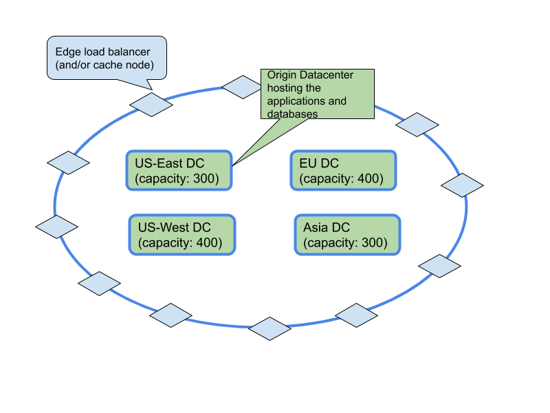
The edge node then needs to determine what origin server to send the request to (assuming there is no caching or cache misses). This is how your typical CDN works, but also how for example, Google and Facebook deliver their applications. In the case of a simple CDN there could be one or more origin servers. In the case of Facebook, the choice is more which of their ‘core’ or ‘larger’ datacenters to send the request to.
With AWS Global Accelerator you can configure listeners (the diamond) in a region to send a certain percentage of traffic to an origin group, ‘Endpoint Groups’ in AWS speak. This is a static configuration, which is not ideal. Additionally, if an origin (the green box in the diagram) reaches its capacity, you will need to update the configuration. This is the part we’re going to make smarter.
In an ideal world, each edge node (the diamond) routes the requests to the closest origin based on the latency between the edge node and the origin. It should also be aware of the total load the origin is under, and how much load the origin can handle. An individual edge node doesn’t know how many other edge nodes there are, and how much each of them is sending each origin. So we need a centralized brain and a feedback loop.
Building a Closed-loop system
To have the system continuously adapt to the changing environment, we need to have access to several operational metrics. We need to know how many requests each edge node (load balancer) is receiving, with that we can infer the total, global, number of incoming requests per second. We also need to know the capacity of each origin since we want to make sure we don’t send more traffic to an origin than it can handle. Finally, we need to know the health and latency between each edge node and each origin. Most of these metrics are dynamic, so we need to continuously publish (or poll) the health information and request per second information.
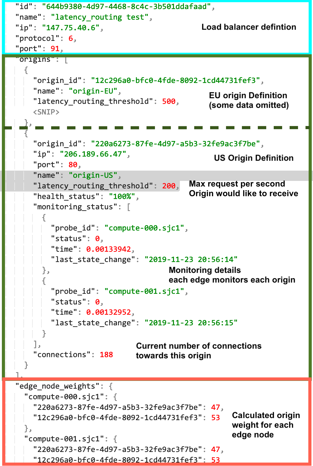
Now that we have all the input data, we can feed this into our software. The software essentially a scheduler, solving a constraint-based assignment problem. The output is a list with all edge nodes and a weight assignment per edge node for each origin. A simple example could look like this:
-Listener 192.0.2.10:443
 - Edge node Amsterdam:
    - Origin EU DC:  90%
    - Origin US-WEST DC:  0%
    - Origin US-EAST DC:  10%
    - Origin Asia DC:  0%
 - Edge node New York:
    - Origin EU DC: 0%
    - Origin US-WEST DC:  0%
    - Origin US-EAST DC:  100%
    - Origin Asia DC:  0%
In the above example for listener 192.0.2.10:443, the Amsterdam edge node will send 90% of the requests to the EU origin, while the remaining 10% is directed to the next closest DC, US-EAST. This means this the EU datacenter is at capacity and is offloading traffic to the next closest origin.
The New York edge node is sending all traffic to the EU-EAST datacenter as there is enough capacity at this point and no need to offload traffic.
Our closed-loop system will re-calculate and publish the results every few seconds so that we can respond to changes quickly.
Let’s start building
I’m going to re-use much of what we’ve built earlier, in this experiment I’m again using Packet.net and their BGP anycast support to build the edge nodes. Please see this blog for details. I’m using Linux LVS as a load balancer for this setup. Each edge node is publishing the needed metrics to prometheus, a time-series database, every 15 seconds. With this, we now have a handful of edge nodes, fully anycasted, and access to all needed metrics per edge node in a centralized system.
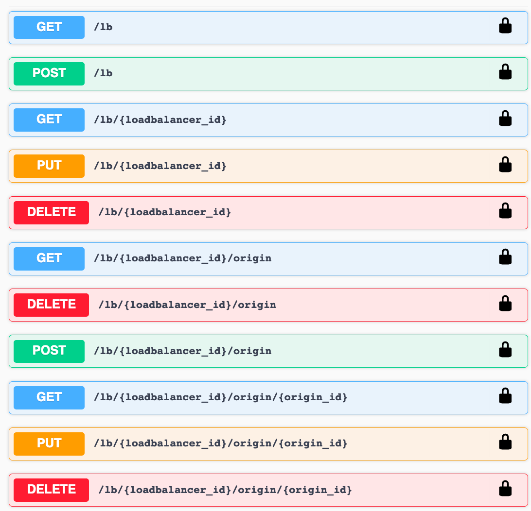
The other thing that is needed is a centralized source of truth. For this, I wrote a Flask based REST API. This API allows us to create new load balancers, add origins, etc. We can also ask this same API for all load balancers, its origins and the health and operational metrics.
The next thing we needed is a script that every few seconds talks to the API to retrieve the latest configuration. With that information, each edge node can update the load balancer configuration, such as create new load balancer listeners and update the origin details such as weight per origin. We now have everything in place and can start testing.
Observations and tuning
I started testing by generating many get requests to one Listener that has two origins, one digitalocean VM in the US and one in Europe. Since all testing was performed from one location, it was hitting one edge datacenter, that has two edge nodes. Those edge nodes would send the traffic to the closest origin, which is the US origin. Now imagine this origin server was hitting its maximum capacity and I want to protect it from being overloaded and start sending some traffic to the other origin. To do that I set the maximum load number for the US origin to 200 requests per second (also see JSON above).
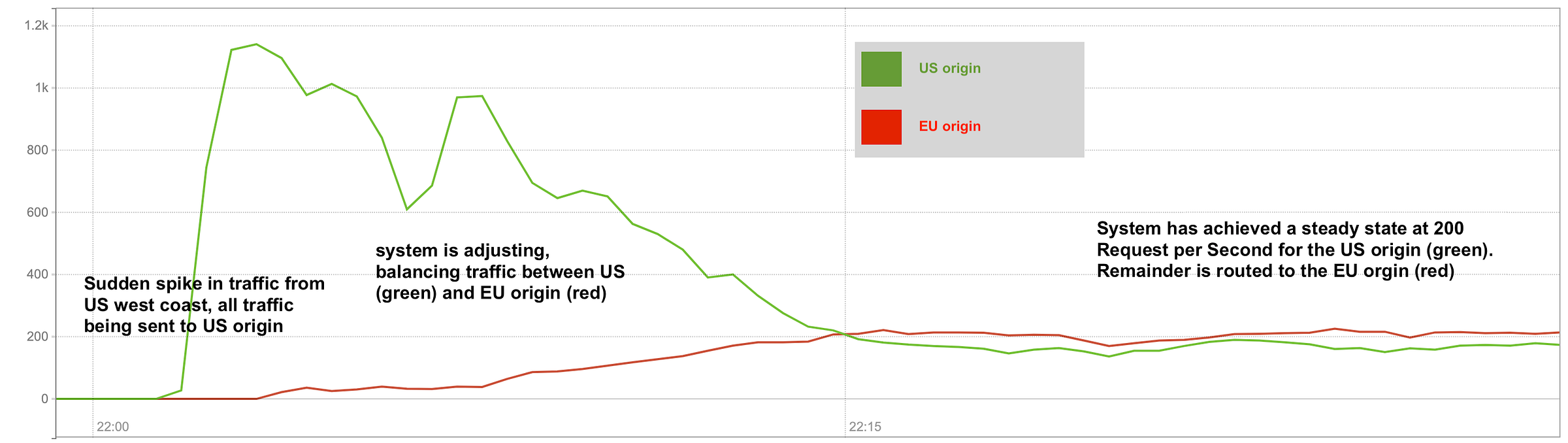
Below you’ll see an interesting visualization of this measurement. At t=0 the total traffic load for both origins is 0, no traffic is coming in at all, which also meant that both origins are well below their max capacity. This means that the US load balancers are configured to send all requests to the US origin as they have the lowest latency and are below the max threshold.
After we generate the traffic, all requests are sent to the US origin to start. As the metrics start coming in the system detects that the total number of incoming requests is exceeding 200, as a result, the load balancer configuration will be updated to start sending traffic to both origin servers, with the intent to not send more than 200 requests per second to the US origin.
Speed vs. accuracy.
One of the things we want to prevent is big sudden swings in traffic. To achieve that I built in a dampening factor that limits the load shifting (ie. load balancer configuration) change to 2 percent per origin for each 15-second interval. Note; that if you have two origins, this means a 2% change per origin, so 4% swing per 15 secsond cycle. This means it will take a bit longer for the system to respond to major changes but will give us substantially more stability, meaning less oscillation between origins and will allow for the system to stabilize. In my initial version, I had no dampening and the system never stabilized and showed significant unwanted sudden traffic swings.
The graph shows an interesting side effect of my testing setup. Since I’m testing from the US west coast and start offloading more and more requests to the EU origin, this means that on average, a single curl will take longer due to the increased round trip time. As a result, the total number of requests goes down. Which is fun, because it means the software needs to adapt constantly. Every time we change the origin weights slightly, the total number or requests changes slightly. This causes some oscillation, but it’s also exactly the oscillation a closed-loop system is designed for, and it works well as long as we have a dampening factor. It also shows that in some instances the total number of inbound requests increases if your website (or any app) is responding faster. Though I’m not sure if that’s representative of a real-world scenario. Still, this was a fun side effect that put a bit of extra stress on the software.
Closing thoughts
This project was fun as it allowed me to combine several of my interests. One of them is global traffic engineering, ie. how do we get traffic to where we’d like it to be processed. We also go to re-use the lessons learned and experience gained from a few of the previous blog posts, specifically how to build anycasted applications with Packet and a deep-dive into AWS Global Accelerator. I got to improve my Python skills by building a Restful API in Flask and make sure it was properly documented using the OpenAPI spec.
Finally, building the actual scheduler was a fun challenge, and it took me a while to figure out how to best solve the assignment problem before I was really happy with the outcome. The result is what could be a Smarter Global Accelerator.